Welcome to pyESMDA’s documentation!#
pyESMDA#











🐍 A python impementation of the famous Ensemble Smoother with Multiple Data Assimilation (ESMDA).
pyesmda is an open-source, and object-oriented library that provides a user friendly implementation of one of the most popular ensemble based method for parameters estimation and data assimilation: the Ensemble Smoother with Multiple Data Assimilation (ES-MDA) algorithm, introduced by Emerick and Reynolds [1-2].
Thanks to its simple formulation, ES-MDA of Emerick and Reynolds (2012) is perhaps the most used iterative form of the ensemble smoother in geoscience applications.
The complete and up to date documentation can be found here: https://pyesmda.readthedocs.io.
🚀 Quick start#
To install pyesmda, the easiest way is through pip:
pip install pyesmda[examples]
Or alternatively using conda
conda install pyesmda[examples]
You might also clone the repository and install from source
pip install -e .[examples]
Once the installation is done, the ESMDA interface is ready to use. Let’s illustrate
how to use the lib with is a simple example where amplitude and change factor parameters
of n exponential function are estimated:
import numpy as np
from pyesmda import ESMDA, ESMDA_RS, ESMDA_DMC, ESMDAInversionType, FixedLocalization
import logging
import scipy as sp

# set logging level
logging.basicConfig(level=logging.INFO)

def exponential(p, x):
    """
    Simple exponential function with an amplitude and change factor.

    Parameters
    ----------
    p : tuple, list
        Parameters vector: amplitude i.e. initial value and change factor.
    x : np.array
        Independent variable (e.g. time).

    Returns
    -------
    np.array
        Result.

    """
    return p[0] * np.exp(x * p[1])


def forward_model(m_ensemble, x):
    """
    Wrap the non-linear observation model (forward model).

    Function calling the non-linear observation model (forward model).
    for all ensemble members and returning the predicted data for
    each ensemble member.

    Parameters
    ----------
    m_ensemble : np.array
        Initial ensemble of N_{e} parameters vector..
    x : np.array
        Independent variable (e.g. time).

    Returns
    -------
    d_pred: np.array
        Predicted data for each ensemble member.
    """
    # Initiate an array of predicted results.
    d_pred = np.zeros([x.shape[0], m_ensemble.shape[1]])
    for j in range(m_ensemble.shape[1]):
        # Calling the forward model for each member of the ensemble
        d_pred[:, j] = exponential(m_ensemble[:, j], x)
    return d_pred

    # seed for the reproductibility
    seed = 0
    rng = np.random.default_rng(seed=seed)

    # a and b are the reference parameters that we look for
    a = 10.0
    b = -0.0020
    # timesteps
    x = np.arange(500)
    # Generate synthetic data used as observations
    obs = exponential((a, b), x) + rng.normal(0.0, 1.0, 500)
The optimal solution (a, b) can be found following:
# Initiate an ensemble of (a, b) parameters
n_ensemble = 100  # size of the ensemble
# Uniform law for the parameter a ensemble
ma = rng.uniform(low=-10.0, high=50.0, size=n_ensemble)
# ma = rng.normal(loc=20.0, scale=20.0, size=n_ensemble)
# Uniform law for the parameter b ensemble
mb = rng.uniform(low=-0.001, high=0.01, size=n_ensemble)
# mb = rng.normal(loc=-.002, scale=.005, size=n_ensemble)
# Prior ensemble
m_ensemble = np.stack((ma, mb), axis=0)

# Observation error covariance matrix
A = rng.normal(loc=0, scale=0.25, size=((obs.size, obs.size)))
# make it PSD by adding strong weight on the diagonal
A.flat[:: A.shape[0] + 1] += 15.0
# perform cholesky factorization
cov_obs = covmats.CovViaCholesky(sp.linalg.cholesky(A, lower=True))

# Bounds on parameters (size m * 2)
m_bounds = np.array([[0.0, 50.0], [-1.0, 1.0]])

# Number of assimilations
n_assimilations = 4

# Use a geometric suite (see procedure un evensen 2018) to compte alphas.
# Also explained in Torrado 2021 (see her PhD manuscript.)
cov_obs_inflation_geo = 1.2
cov_obs_inflation_factors: list[float] = [1.1]
for l in range(1, n_assimilations):
    cov_obs_inflation_factors.append(
        cov_obs_inflation_factors[l - 1] / cov_obs_inflation_geo
    )
scaling_factor: float = np.sum(1 / np.array(cov_obs_inflation_factors))
cov_obs_inflation_factors = [
    alpha * scaling_factor for alpha in cov_obs_inflation_factors
]

np.testing.assert_almost_equal(sum(1.0 / np.array(cov_obs_inflation_factors)), 1.0)

# This is just for the test
cov_mm_inflation_factor = 1.2

solver = ESMDA(
    obs,
    m_ensemble,
    cov_obs,
    forward_model,
    forward_model_args=(x,),
    forward_model_kwargs={},
    n_assimilations=n_assimilations,
    cov_obs_inflation_factors=cov_obs_inflation_factors,
    cov_mm_inflation_factor=cov_mm_inflation_factor,
    m_bounds=m_bounds,
    save_ensembles_history=True,
    inversion_type=ESMDAInversionType.CHOLESKY,
    random_state=seed,
    truncation=0.99,
    logger=logging.getLogger("ESMDA"),
)
# Call the ES-MDA solver
solver.solve()

# Assert that the parameters are found with a 5% accuracy.
assert np.isclose(np.average(solver.m_posterior, axis=1), np.array([a, b]), rtol=5e-2).all()

# Get the approximated parameters
a_approx, b_approx = np.average(solver.m_posterior, axis=1)

# Get the uncertainty on the parameters
a_std, b_std = np.sqrt(np.diagonal(solver.cov_mm))


solver.logger.info(f"a = {a_approx:.5f} +/- {a_std:.4E}")
solver.logger.info(f"b = {b_approx:.5f} +/- {b_std: 4E}")
Which yields
INFO:ESMDA:Assimilation # 1
INFO:ESMDA:Assimilation # 2
INFO:ESMDA:Assimilation # 3
INFO:ESMDA:Assimilation # 4
INFO:ESMDA:a = 9.99314 +/- 1.3697E-01
INFO:ESMDA:b = -0.00202 +/-  7.707785E-05
In the above example, the user has to define the number of assimilations as well as the inflation factor(s). pyesmda implement two automatic variant of ESMDA, namely the restricted step variant [3] through`ESMDA_RS` and the data misfit controller variant [4] through ESMDA_DMC:
# Example with ESMDA_RS: no inflation factor provided nor number of assimilations

# A priori estimated parameters covariance
std_m_prior = np.array([30.0, 0.01])

# This is just for the test
cov_mm_inflation_factor: float = 0.9

solver = ESMDA_RS(
    obs,
    m_ensemble,
    cov_obs,
    forward_model,
    forward_model_args=(x,),
    forward_model_kwargs={},
    cov_mm_inflation_factor=cov_mm_inflation_factor,
    m_bounds=m_bounds,
    C_MD_localization=FixedLocalization(np.ones((m_ensemble.shape[0], obs.size))),
    C_DD_localization=FixedLocalization(np.ones((obs.size, obs.size))),
    save_ensembles_history=True,
    std_m_prior=std_m_prior,
    random_state=123,
    batch_size=1,
    is_parallel_analyse_step=True,
    logger=logging.getLogger("ESMDA-RS"),
)
# Call the ES-MDA-RS solver
solver.solve()

# Assert that the parameters are found with a 5% accuracy.
assert np.isclose(np.average(solver.m_posterior, axis=1), np.array([a, b]), rtol=1e-1).all()

# Get the approximated parameters
a_approx, b_approx = np.average(solver.m_posterior, axis=1)

# Get the uncertainty on the parameters
a_std, b_std = np.sqrt(np.diagonal(solver.cov_mm))


solver.logger.info(f"a = {a_approx:.5f} +/- {a_std:.4E}")
solver.logger.info(f"b = {b_approx:.5f} +/- {b_std: 4E}")
Which yields:
INFO:ESMDA-RS:- Inflation factor = 4132.540
INFO:ESMDA-RS:Assimilation # 2
INFO:ESMDA-RS:- Inflation factor = 62.403
INFO:ESMDA-RS:Assimilation # 3
INFO:ESMDA-RS:- Inflation factor = 9.042
INFO:ESMDA-RS:Assimilation # 4
INFO:ESMDA-RS:- Inflation factor = 1.145
INFO:ESMDA-RS:a = 9.81329 +/- 1.5023E-01
INFO:ESMDA-RS:b = -0.00190 +/-  7.620613E-05
And here is how to use ESMDA_DMC:
# Note: no inflation factor provided nor number of assimilations
# This is just for the test
cov_mm_inflation_factor: float = 0.9

solver = ESMDA_DMC(
    obs,
    m_ensemble,
    cov_obs,
    forward_model,
    forward_model_args=(x,),
    forward_model_kwargs={},
    cov_mm_inflation_factor=cov_mm_inflation_factor,
    m_bounds=m_bounds,
    C_MD_localization=FixedLocalization(np.ones((m_ensemble.shape[0], obs.size))),
    C_DD_localization=FixedLocalization(np.ones((obs.size, obs.size))),
    save_ensembles_history=True,
    random_state=123,
    batch_size=1,
    is_parallel_analyse_step=True,
    logger=logging.getLogger("ESMDA-DMC"),
)
# Call the ES-MDA-RS solver
solver.solve()

# Assert that the parameters are found with a 5% accuracy.
assert np.isclose(np.average(solver.m_posterior, axis=1), np.array([a, b]), rtol=5e-2).all()

# Get the approximated parameters
a_approx, b_approx = np.average(solver.m_posterior, axis=1)

# Get the uncertainty on the parameters
a_std, b_std = np.sqrt(np.diagonal(solver.cov_mm))


solver.logger.info(f"a = {a_approx:.5f} +/- {a_std:.4E}")  # ty:ignore[possibly-missing-attribute]
solver.logger.info(f"b = {b_approx:.5f} +/- {b_std: 4E}")  # ty:ignore[possibly-missing-attribute]
Which yields:
INFO:ESMDA-DMC:Assimilation # 2
INFO:ESMDA-DMC:- Inflation factor = 661.601
INFO:ESMDA-DMC:Assimilation # 3
INFO:ESMDA-DMC:- Inflation factor = 181.950
INFO:ESMDA-DMC:Assimilation # 4
INFO:ESMDA-DMC:- Inflation factor = 12.253
INFO:ESMDA-DMC:Assimilation # 5
INFO:ESMDA-DMC:- Inflation factor = 1.097
INFO:ESMDA-DMC:a = 9.78691 +/- 1.3310E-01
INFO:ESMDA-DMC:b = -0.00191 +/-  6.493808E-05
See all use cases in the tutorials section of the documentation.
2D example#
To illustrate more of pyesmda, let’s use a toy 2D example. The forward is simple static smoohting (non linear but with no time dependance) and is used both to produce a reference field from which observations will be sampled and the inversion.
Import the required modules
import matplotlib.pyplot as plt
import numpy as np
import scipy as sp
import covmats
import pyesmda
from pyesmda._utils import NDArrayFloat
import logging
import nested_grid_plotter as ngp
Apply nice parameters for the plots
ngp.apply_nice_default_rc_params()
Create some logging.Logger instances to illustrate how to use them in a complex workflow
# Create loggers
main_logger = logging.getLogger("main")
main_logger.setLevel(logging.INFO)
esmda_logger = logging.getLogger("ESMDA")
esmda_logger.setLevel(logging.INFO)
main_logger.info("This is the main logger")
esmda_logger.info("This is the ESMDA logger")
Let’s use an example provided by covmats. Here, the prior covariance matrix, $mathbf{C}_{mathrm{prior}}$ is represented as a sparse factorization of its inverse $mathbf{C}_{mathrm{prior}}^{-1}$ with $mathbf{LDL}^{mathrm{T}} = mathbf{PC}_{mathrm{prior}}^{-1}mathbf{P}^{mathrm{T}}$. This is wrapped in the covmats.CovViaSparsePrecisionCholesky` instance we create:
cov_prior = covmats.CovViaSparsePrecisionCholesky(
    covmats.load_precision_example_4225x_SCF()
)
cov_prior
<4225x4225 CovViaSparsePrecisionCholesky with dtype=float64>
The covariance matrix has shape (4225, 4225) , let’s define a square domain (65, 65) and perform a non conditional simulation using our prior. We set a mean @ 50 and display it:
# Domain dimensions
nx = ny = int(np.sqrt(cov_prior.shape[0]))

# Non conditonal simulation -> change the random states (seeds) to obtain different fields
simu_ = cov_prior.sample_mvnormal(shape=(1,), random_state=2026).reshape(ny, nx).T
mean= 50.0
# Reference field
s_ref = np.abs(simu_ + mean)
# Initial guess
s_init = np.abs(cov_prior.sample_mvnormal(shape=(1,), random_state=15653).reshape(ny, nx).T)

plotter = ngp.Plotter(fig=plt.figure(figsize=(9, 4.3)),builder=ngp.SubplotsMosaicBuilder([["ax11", "ax12"]], sharex=True, sharey=True))
ngp.multi_imshow(
    plotter.axes,
    plotter.fig,
    data={"Reference": s_ref, "Initial guess": s_init},
    xlabel="X", ylabel="Y", imshow_kwargs=dict(cmap=plt.get_cmap("jet"),
    aspect="equal",
    vmin=0.0,
    vmax=120,)
)
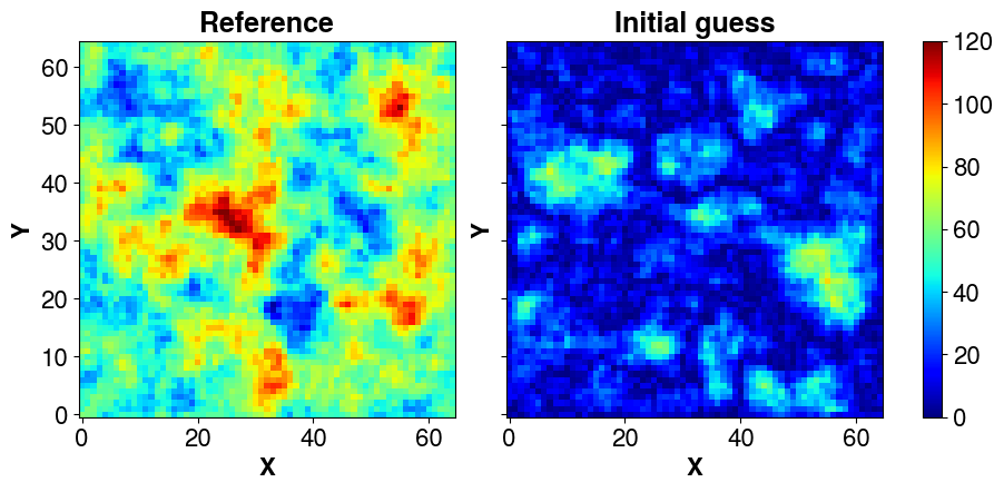
The forward is simple static smoohting (non linear but with no time dependance) and is used both to produce a reference field from which observations will be sampled and the inversion. Here, forward_multiple is just the generalization to an ensemble of vectors, i.e., in ESMDA, most forward calls for an iteration can be performed in parallel. But it is the responsibility of the user to decide and implement the sequential forward computation (a simple for loop as here) or the parallelized computation (with mpi, multiprocessing, joblib or whatever tool that suits best).
# Data transform operator
def transform_model(x: NDArrayFloat) -> NDArrayFloat:
    """Transform the input space into the output space."""
    return sp.ndimage.gaussian_filter(4.0 * x**2, sigma=2.0)

# Sampling operator
def sample_d(d: NDArrayFloat, sampling_fraction: float = 0.05) -> NDArrayFloat:
    """
    Sample within a vector.

    Parameters
    ----------
    d : NDArrayFloat
        Values to sample.
    sampling_fraction : float, optional
        Fraction of the values to sample, by default 0.05.
    """
    return d.ravel("F")[:: int(d.size / (sampling_fraction * 1000))]

def forward(x: NDArrayFloat) -> NDArrayFloat:
    """
    Forward model (data transform + sampling in the output space).

    Parameters
    ----------
    x : NDArrayFloat
        Input parameters vector with size (N_s).

    Returns
    -------
    NDArrayFloat
    """
    return sample_d(transform_model(x))

def forward_multiple(X: NDArrayFloat, *args, **kargs) -> NDArrayFloat:
    """
    Return the results of the forward for an ensemble of input vectors.

    Parameters
    ----------
    X : _type_
        Input vectors as a matrix with size (N_s, N_e), N_s being the number of
        parameter values per vector and N_e the number of vectors, aka the ensemble
        size.

    Returns
    -------
    NDArrayFloat
        _description_
    """
    res = []
    _X = np.atleast_2d(X.T)
    for i in range(_X.shape[0]):
        res.append(forward(_X[i, :].reshape(nx, ny, order="F")))
    return np.vstack(res).T

# The input vector much match a flatten version of the field (Here, 2D -> 1D).
obs = forward_multiple(s_ref.ravel())[:, 0]
# Some test to check that all works as expected
s_ens = np.vstack([s_ref.ravel("F"), s_init.ravel("F")]).T
assert s_ens.shape == (nx * ny, 2)
d_pred = forward_multiple(s_ens)
assert d_pred.shape == (obs.size, 2)
np.testing.assert_almost_equal(d_pred[:, 0], obs)
Define the covariance matrix of observation errors (cov_obs). To illustrate a complex case, the matrix is assumed non diagonal.
n = np.size(obs)
amplitude = (np.max(obs) - np.min(obs))

# CASE 1: diagonal covariance matrix (this is the simplest case)
# 10% error on the observations
# cov_obs = covmats.CovViaDiagonal(
#     np.ones(n) * amplitude ** 2
# )

# CASE 2: non diagonal through Cholesky
L = np.zeros((n ,n), dtype=np.float64)
# Add some random non-zero covariances
for i in range(n):
    for j in range(i + 1, n):
        if np.random.rand() < 0.1:  # 10% chance of non-zero covariance
            cov = np.random.uniform(-0.05, 0.05) * amplitude
            L[i, j] = cov
            L[j, i] = cov  # symmetry
# Add non zero diagonal
L.flat[:: n + 1] = amplitude * 0.1
# Make it lower triangular and define the covariance as a cholesky factorization
cov_obs = covmats.CovViaCholesky(np.tril(L))

# Show the dense matrix
plt.imshow(cov_obs.todense())
plt.colorbar()
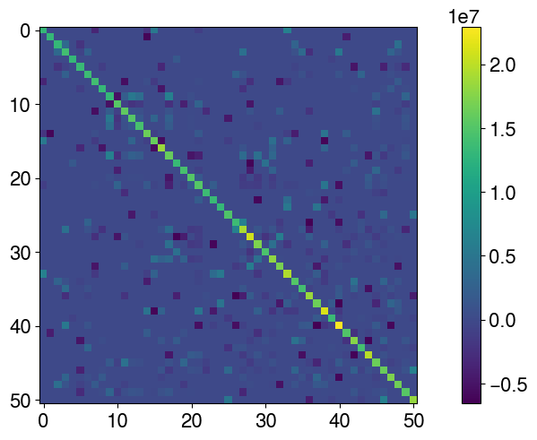
Perturb the observations to avoid the inverse crime (using the same forward to generate the synthetic data and perform the inversion makes the problem well posed and simple to solve. Adding noise mitigates it a bit).
obs_perturb = (
    obs + cov_obs.sample_mvnormal([1], random_state=np.random.default_rng(2151))[0]
)
# Plot the non perturbed observations vs perturbed ones
# The perturbed ones will be used for the inversion
pl = ngp.Plotter()
lims = (np.min(obs), np.max(obs))
diff = lims[1] - lims[0]
lims = (lims[0]- 0.2 * diff, lims[1]+ 0.2 * diff)
pl.axes[0].plot(lims, lims, color="r")
pl.axes[0].scatter(obs_perturb, obs)
pl.axes[0].set_xlabel("Perturbed values (observations)")
pl.axes[0].set_ylabel("Values")
pl.axes[0].set_aspect("equal")
pl.axes[0].set_xlim(lims)
pl.axes[0].set_ylim(lims)
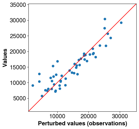
The next step is to “factorize” the parameters covariance matrix using an ensemble. For this, we rely on covmats. The number of members is set to 200.
ens_mat = covmats.CovViaEnsemble(cov_prior.sample_mvnormal((200,), random_state=2026))
assert ens_mat.n_pts == 4225
Create the ESMDA instance
solver = pyesmda.ESMDA(
    obs=obs_perturb,
    m_init=np.abs(ens_mat.ensemble.T + 25.0),
    cov_obs=cov_obs,
    forward_model=forward_multiple,
    n_assimilations=6,
    random_state=2026,
    logger=esmda_logger,
    inversion_type=pyesmda.ESMDAInversionType.WOODBURY,
)
# Sanity checks just for the tests
assert solver.m_dim == 4225
assert solver.d_dim == obs.size
Run the inversion process
solver.solve()
INFO:ESMDA:Assimilation # 1
INFO:ESMDA:Assimilation # 2
INFO:ESMDA:Assimilation # 3
INFO:ESMDA:Assimilation # 4
INFO:ESMDA:Assimilation # 5
INFO:ESMDA:Assimilation # 6
INFO:ESMDA:Forecast for the final ensemble
The solver produces the a posterori ensemble which we can compute the mean => Plot the inverted field versus the reference one (in real world applications, the refrence is not know).
plotter = ngp.Plotter(
    plt.figure(figsize=(9.0, 4.4), constrained_layout=True),
    builder=ngp.SubplotsMosaicBuilder([["ref", "inv"]]),
)

ngp.multi_imshow(
    plotter.axes,
    data={
        "Reference": s_ref.T,
        "Mean Post inv": solver.m_posterior.mean(-1).reshape(nx, ny, order="F").T,
    },
    fig=plotter.fig,
    imshow_kwargs=dict(
        origin="lower",
        cmap=plt.get_cmap("jet"),
        aspect="equal",
        vmin=0.0,
        vmax=120,
    ),
    cbar_kwargs=dict(pad=0.01),
)
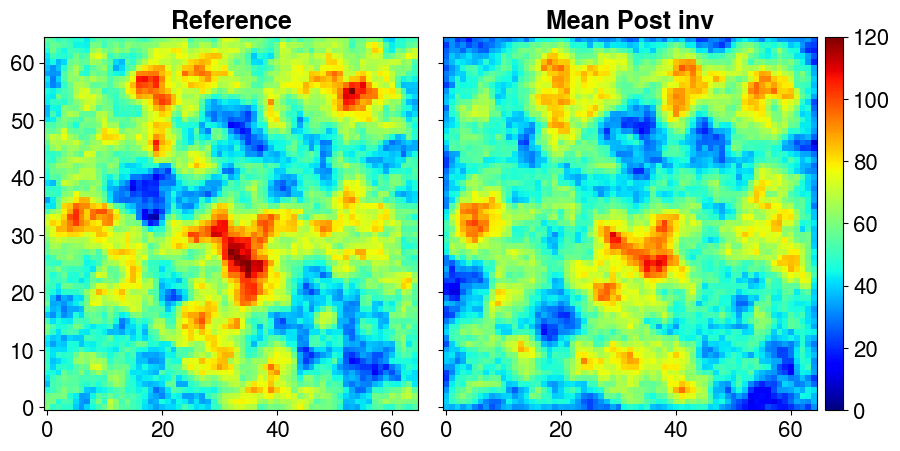
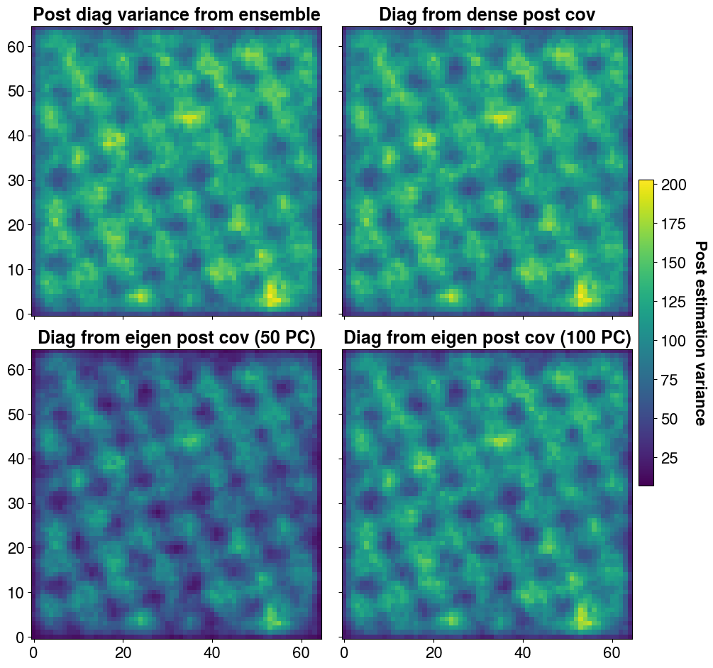
This posterior ensemble also allows obtaining a low-rank approximation of the posterior covariance matrix. One can then extract the estimation variance. It is also possible to convert this low-rank matrix into another factorization, such as for example Eigen: in the present case, we construct the Eigen matrix with 50 and then with 100 principal components to compare the effects. We also construct the dense matrix (which is not possible for large-scale problems) for comparison.
post_cov_ens = covmats.CovViaEnsemble(solver.m_posterior.T)
post_cov_dense = post_cov_ens.todense()
post_cov_50_pc = covmats.eigen_factorize_cov_mat(post_cov_ens, n_pc=50)
post_cov_100_pc = covmats.eigen_factorize_cov_mat(post_cov_ens, n_pc=100)
The higher the number of realizations or PC, the better the approximation of the posterior variance
plotter = ngp.Plotter(
    plt.figure(figsize=(10.0, 9.3), constrained_layout=True),
    builder=ngp.SubplotsMosaicBuilder([["diag", "dense"], ["50pc", "100pc"]]),
)

ngp.multi_imshow(
    plotter.axes,
    data={
        "Post diag variance from ensemble": post_cov_ens.get_diagonal()
        .reshape(nx, ny, order="F")
        .T,
        "Diag from dense post cov": np.diagonal(post_cov_dense)
        .reshape(nx, ny, order="F")
        .T,
        "Diag from eigen post cov (50 PC)": post_cov_50_pc.get_diagonal()
        .reshape(nx, ny, order="F")
        .T,
        "Diag from eigen post cov (100 PC)": post_cov_100_pc.get_diagonal()
        .reshape(nx, ny, order="F")
        .T,
    },
    fig=plotter.fig,
    imshow_kwargs=dict(
        origin="lower",
        cmap=plt.get_cmap("viridis"),
        aspect="equal",
    ),
    cbar_kwargs=dict(pad=0.01, shrink=0.5),
    cbar_title="Post estimation variance",
)
With ESMDA, the final (posterior) ensemble already allows estimating the estimation variance on the searched parameters and on the predictions.
nrows = 5
ncols = 5
plotter = ngp.Plotter(
    plt.figure(figsize=(10.0, 9.3), constrained_layout=True),
    builder=ngp.SubplotsMosaicBuilder(
        [[f"ax{i}-{j}" for i in range(nrows)] for j in range(ncols)],
        sharex=True,
        sharey=True,
    ),
)

ngp.multi_imshow(
    plotter.axes,
    data={
        f"r#{i}": solver.m_posterior[:, i].reshape(nx, ny, order="F").T
        for i in range(nrows * ncols)
    },
    fig=plotter.fig,
    imshow_kwargs=dict(
        origin="lower",
        cmap=plt.get_cmap("jet"),
        aspect="equal",
    ),
    cbar_kwargs=dict(pad=0.01, shrink=0.5),
    cbar_title="Parameter value",
)
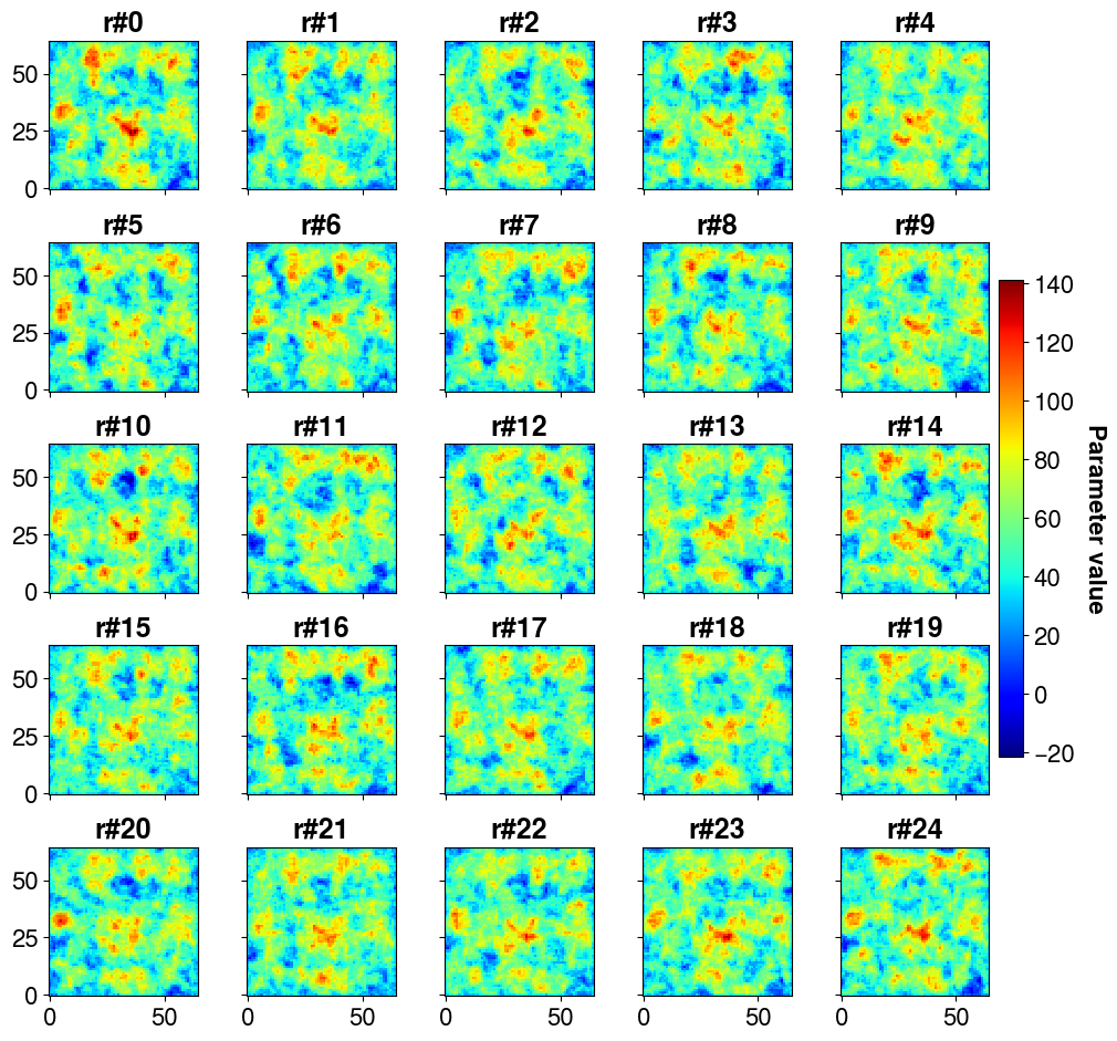
But it should be noted that the interest of having the posterior covariance matrix (of inverted parameter values) is that it is possible to draw samples (realizations) from it and thus generate new ensembles to quantify the uncertainty on predictions (at the cost of one forward call per sample).
# make 200 posterior realizations => we sample from post_cov_ens
post_samples_200 = (
    solver.m_posterior.mean(-1).T
    + post_cov_ens.sample_mvnormal(shape=(200,), random_state=solver.rng)
).T
post_samples_200.shape
(4225, 200)
Let’s plot the first 25 “new” realizations
nrows = 5
ncols = 5
plotter = ngp.Plotter(
    plt.figure(figsize=(10.0, 9.3), constrained_layout=True),
    builder=ngp.SubplotsMosaicBuilder(
        [[f"ax{i}-{j}" for i in range(nrows)] for j in range(ncols)],
        sharex=True,
        sharey=True,
    ),
)

ngp.multi_imshow(
    plotter.axes,
    data={
        f"r#{i}": post_samples_200[:, i].reshape(nx, ny, order="F").T
        for i in range(nrows * ncols)
    },
    fig=plotter.fig,
    imshow_kwargs=dict(
        origin="lower",
        cmap=plt.get_cmap("jet"),
        aspect="equal",
    ),
    cbar_kwargs=dict(pad=0.01, shrink=0.5),
    cbar_title="Parameter value",
)
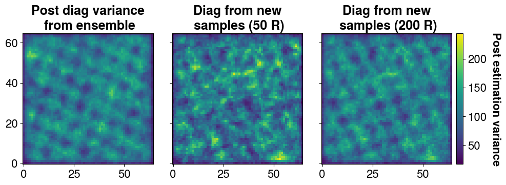
It is possible to find the variance back from the ensemble (or a sub ensemble). The more samples, the more accurate.
plotter = ngp.Plotter(
    plt.figure(figsize=(10.0, 3.5), constrained_layout=True),
    builder=ngp.SubplotsMosaicBuilder([["diag", "50pc", "ens"]]),
)

ngp.multi_imshow(
    plotter.axes,
    data={
        "Post diag variance\n from ensemble": post_cov_ens.get_diagonal().reshape(
            nx, ny, order="F"
        ),
        "Diag from new\n samples (50 R)": covmats.CovViaEnsemble(
            post_samples_200[:, :50].T
        )
        .get_diagonal()
        .reshape(nx, ny, order="F")
        .T,
        "Diag from new\n samples (200 R)": covmats.CovViaEnsemble(post_samples_200.T)
        .get_diagonal()
        .reshape(nx, ny, order="F")
        .T,
    },
    fig=plotter.fig,
    imshow_kwargs=dict(
        origin="lower",
        cmap=plt.get_cmap("viridis"),
        aspect="equal",
    ),
    cbar_kwargs=dict(pad=0.01),
    cbar_title="Post estimation variance",
)
🛠️ Failure Handling in ESMDA#
ESMDA was initially developed in the context of porosity and permeability inversion for reservoir exploitation in oil and gas (ERT, Black-oil Model, reactive transport, …). It is frequent that some simulations do not converge due to non-convergence issues. This is why pyesmda is equipped with a mechanism allowing to accept some losses during computation.
Setting the Maximum Failure Fraction#
When initializing the ESMDA solver, specify the max_failure_fraction parameter:
solver = ESMDABase(
    obs=observations,
    m_init=initial_parameters,
    cov_obs=observation_covariance,
    forward_model=your_forward_model,
    max_failure_fraction=0.1,  # Allow up to 10% of ensemble members to fail
    ...
)
Parameter values:
max_failure_fraction= 0.0 (default): No failures tolerated — any failed member raises an exception immediately (strict behavior)
max_failure_fraction= 0.1: Allow up to 10% of the initial ensemble to fail
max_failure_fraction= 0.5: Allow up to 50% of the initial ensemble to fail
What Constitutes a “Failed” Member#
A member is considered failed if its prediction vector contains at least one NaN value. This typically occurs when:
The forward model (reservoir simulation) did not converge
Physical constraints were violated
Numerical instabilities occurred
Monitoring Failed Members#
After running the solver, you can check the failure status:
# Number of excluded members
n_failed = solver.n_excluded_members

# Indices of failed members (in the original ensemble)
failed_indices = solver.excluded_member_indices

# Current failure fraction
current_fraction = solver.failure_fraction

# Indices of still-active members
active_indices = solver.active_member_indices
Automatic Exclusion Behavior#
When a member fails:
It is automatically removed from both m_posterior (parameters) and d_pred (predictions)
The failed member’s original index is recorded in _excluded_member_indices
The active members continue the assimilation process
If the cumulative failure fraction exceeds max_failure_fraction, an exception is raised and the solver stops
Key Properties#
solver.active_member_indices      # Returns indices of non-failed members
solver.excluded_member_indices    # Returns indices of failed members
solver.n_excluded_members         # Returns count of failed members
solver.failure_fraction           # Returns fraction of failed members
solver.max_failure_fraction       # The tolerance threshold
Example Usage#
# Initialize with 20% failure tolerance
solver = ESMDABase(
    obs=obs,
    m_init=m_init,
    cov_obs=cov_obs,
    forward_model=forward_model,
    max_failure_fraction=0.2,  # Allow up to 20% to fail
    n_assimilations=4,
    ...
)

# Run the solver
solver.solve()

# Check results
print(f"Initial ensemble size: {solver._initial_n_ensemble}")
print(f"Failed members: {solver.n_excluded_members}")
print(f"Failure fraction: {solver.failure_fraction:.1%}")
print(f"Active members: {len(solver.active_member_indices)}")
This mechanism is essential for practical reservoir simulation applications where convergence failures are common and should not halt the entire inversion process.
🛠️ Localization#
Here are some of the cool features that this implementation provides (to the best of our knowledge in 2025).
🏗️ Complete example with supporting paper coming Q1 2027.
TODO:link to correlation matrices building
TODO:link to example with localization
See all use cases in the tutorials section of the documentation.
🔑 License#
This project is released under the BSD 3-Clause License.
Copyright (c) 2021-2026, Antoine COLLET. All rights reserved.
For more details, see the LICENSE file included in this repository.
⚠️ Disclaimer#
This software is provided “as is”, without warranty of any kind, express or implied, including but not limited to the warranties of merchantability, fitness for a particular purpose, or non-infringement. In no event shall the authors or copyright holders be liable for any claim, damages, or other liability, whether in an action of contract, tort, or otherwise, arising from, out of, or in connection with the software or the use or other dealings in the software.
By using this software, you agree to accept full responsibility for any consequences, and you waive any claims against the authors or contributors.
📧 Contact#
For questions, suggestions, or contributions, you can reach out via:
Email: antoinecollet5@gmail.com
GitHub: antoinecollet5/pyesmda
We welcome contributions!
✨ How to Cite#
Software/Code citation for pyESMDA:
Antoine Collet. (2026). pyESMDA - Python Ensemble Smoother with Multiple Data Assimilation (v1.0.0). Zenodo. https://doi.org/10.5281/zenodo.7425670
📚 References#
[1] Emerick, A. A. and A. C. Reynolds, Ensemble smoother with multiple data assimilation, Computers & Geosciences, 2012.
[2] Emerick, A. A. and A. C. Reynolds. (2013). History-Matching Production and Seismic Data in a Real Field Case Using the Ensemble Smoother With Multiple Data Assimilation. Society of Petroleum Engineers - SPE Reservoir Simulation Symposium 1. 2. 10.2118/163675-MS.
[3] Duc Le, Alexandre Emerick, and Albert Reynolds. An Adaptive Ensemble Smoother With Multiple Data Assimilation for Assisted History Matching. SPE Journal, June 2016. doi:10.2118/173214-PA.
[4] Marco Iglesias and Yuchen Yang. Adaptive regularisation for ensemble Kalman inversion. Inverse Problems, 37(2):025008, January 2021. doi:10.1088/1361-6420/abd29b.
Free software: SPDX-License-Identifier: BSD-3-Clause